The problem
Skin-friction drag comes from a thin layer of slow air near a surface that you can’t see.
Wind tunnel testing · ME 347 · Cal Poly
Friction drag comes from a layer of slowed air too thin to see. With a team of four, I traced airspeed millimeter by millimeter above a flat plate, watched that layer grow, and turned it into a drag estimate.

The problem
Skin-friction drag comes from a thin layer of slow air near a surface that you can’t see.
What I did
Moved a probe up from the plate in small steps at two locations and converted the readings into velocity profiles.
The result
Measured the layer growing from 2.8 mm to 4.5 mm and calculated drag, cross-checked against laminar and turbulent theory.
Stepped a Pitot-static probe away from the plate at two stations.
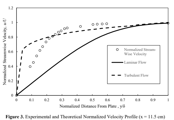
Turned pressure readings into velocity profiles.
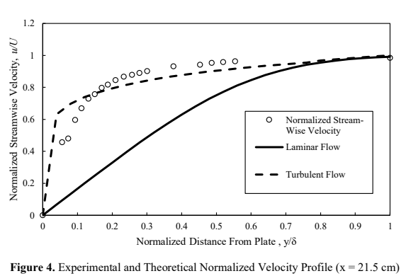
Checked the profiles against laminar and turbulent theory.
Calculated drag from how much momentum the layer lost.
Worked with a team of four on this lab, and I measured the velocity field developing over a flat plate. The profiles let us track boundary-layer growth, calculate displacement and momentum thickness, and compare the resulting drag estimate with laminar and turbulent theory.
Two stations, one developing boundary layer
A Pitot-static tube moved outward from the plate in small increments at x = 11.5 cm and x = 21.5 cm. Manometer deflection was converted to dynamic pressure and local velocity, with the plateau defining the free stream.
The free-stream speed was approximately 20.03 m/s. Boundary-layer thickness was identified where the local velocity reached 99% of that value.
Viscous effects spread farther from the wall
The measured boundary layer grew from 2.775 mm to 4.48 mm between the two stations. Displacement thickness increased from 0.435 mm to 0.582 mm, while momentum thickness increased from 0.194 mm to 0.330 mm.
Those changes are consistent with a developing boundary layer: progressively more fluid is slowed by the wall, increasing both the effective displacement of the outer flow and its momentum deficit.
| Station | Reynolds number | Boundary layer | Displacement | Momentum |
|---|---|---|---|---|
| 11.5 cm | 1.50 × 10⁵ | 2.775 mm | 0.435 mm | 0.194 mm |
| 21.5 cm | 2.80 × 10⁵ | 4.480 mm | 0.582 mm | 0.330 mm |
Measurements fell between ideal laminar and turbulent behavior
At both stations, the experimental profile rose more rapidly than the Blasius laminar solution and followed the turbulent power-law curve more closely through much of the layer. It did not match either ideal model exactly.
A velocity profile becomes a force estimate
Numerical integration of each profile produced momentum thickness, which was then used to estimate plate drag. The calculated drag force increased downstream from 0.00463 N to 0.00788 N as the momentum deficit accumulated.
The drag coefficient remained close to the laminar prediction even though the profile shape appeared more turbulent, reinforcing that the layer was in transition rather than fully developed in either regime.
Model disagreement identified the flow regime
The experimental thickness stayed between the laminar and turbulent predictions, while the velocity shape leaned turbulent and the drag metrics leaned laminar. Together, those results point to a transitional boundary layer. The largest uncertainty came from resolving velocity very near the wall, compounded by wind-tunnel interruptions during the traverse.